CE Board Exam Randomizer

Introduction to Surveying and Discussion of Errors

Surveying is the science of determining the earth's dimensions and surface form by measuring distances, directions, and elevations. It also covers staking out lines/grades for construction and the computation of areas, volumes, and related quantities for preparing maps and diagrams.

Common Tools Used in Surveying

• Common/Traditional: tapes, levels, theodolites, compasses, leveling staffs
• Tech / New Tech: total stations, GNSS/GPS receivers, digital levels, LiDAR, UAVs (drone mapping)

Types of Surveys

Plane vs. Geodetic

• Plane Surveys → Treat the earth as flat; north→south lines assumed parallel. Valid for small areas where curvature is negligible.
• Geodetic Surveys → Adjust for the earth's curvature (used for larger regions/high precision control).

By Purpose

• Land Surveys → Locate property lines; subdivide land; determine land areas; support land transfer.
• Topographic Surveys → Locate and map natural/constructed features with elevations and planimetry.
• Route Surveys → Define relief and locate natural/artificial objects along proposed routes (highways, pipelines, utilities).
• Construction Surveys → Lay out structures and provide elevations/controls during construction.
• Hydrographic Surveys → Chart shorelines; determine underwater topography; estimate stream velocity/flow conditions.
• As-Built Surveys → Document the final positions and dimensions of features after construction.

Quick Reference

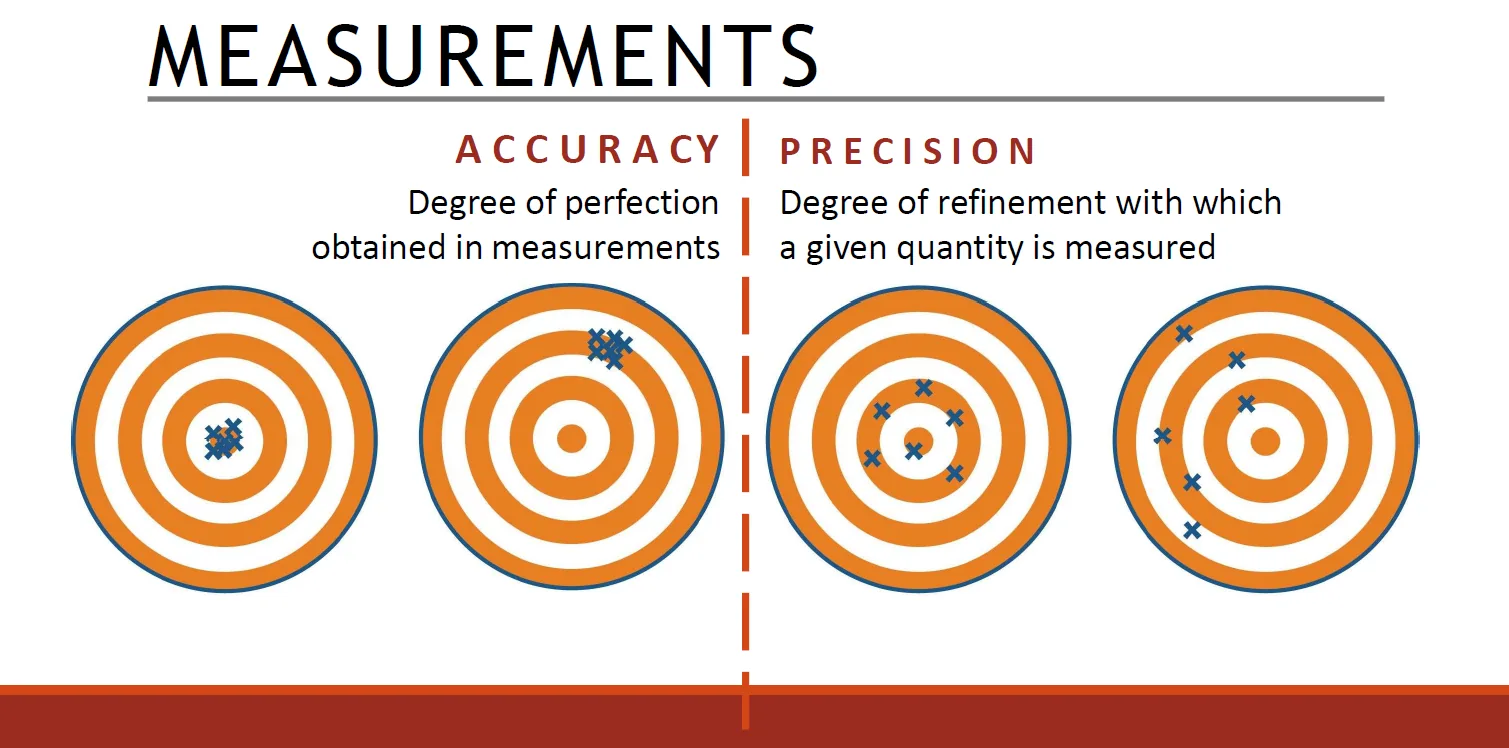
Measurements, Accuracy & Precision

Measurement is central to surveying, but no measurement is exact; the true value is never fully known. Accuracy = closeness to the true value (degree of perfection), while Precision = repeatability or refinement of readings.

Aim: Use skill, judgment, and proper methods to make measurements as accurate and precise as practical.

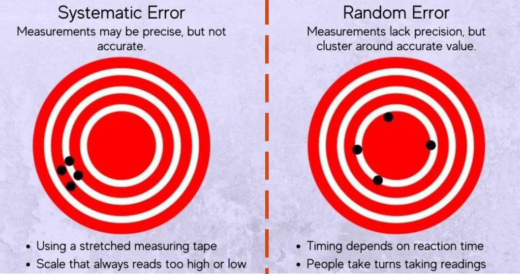
Mistakes vs. Errors

• Mistake (Blunder): due to inattention or misunderstanding; eliminable by careful checking.
• Error (Unavoidable): due to limits of senses, instrument imperfections, or environment; cannot be eliminated but can be minimized.

Relative / Probable Error

835.82 ± 0.06

The quality of a measurement can be expressed by stating a relative error.

Maximum Probable Value: 835.88ft

Minimum Probable Value: 835.76ft

Most Probable Value: 835.82ft

Treating a Set of Repeated Measurements

1. Arithmetic Mean (assumed best/most-probable value):  $\,\mu=\dfrac{\sum x_i}{n}\,$
2. Residuals (deviations):  $\,v_i=x_i-\mu\,$
3. Standard Deviation (sample):  $\,\sigma=\sqrt{\dfrac{\sum v_i^{2}}{n-1}}$
   Why $n-1$? Imagine you're measuring how much students deviate from the class average — but you don't know the true class average, so you use your group's average. Since your group average is “tuned” to your group's own values, your spread will look smaller. Dividing by $n-1$ counteracts that, making the estimate closer to the true population spread.
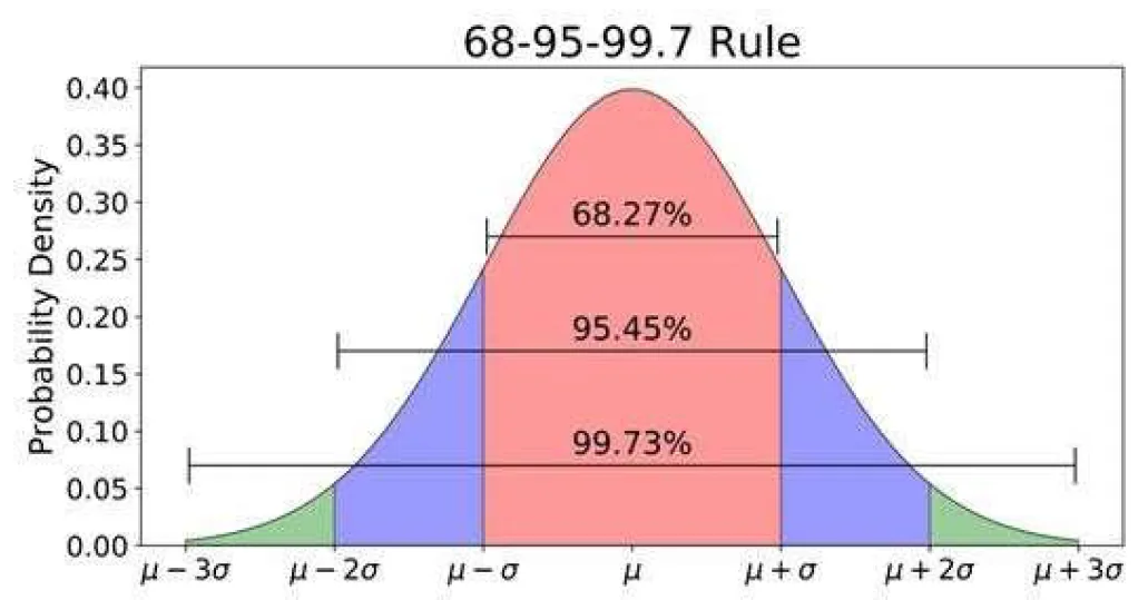
4. Probability (Normal) Curve insights:
   • There is 68.27% chance that the error is $\pm\sigma$ or less and 31.73% chance that the error is larger.
   • There is 95.45% chance that the error is $\pm2\sigma$ or less and 4.55% chance that the error is larger.
   • There is 99.73% chance that the error is $\pm3\sigma$ or less and 0.27% chance that the error is larger.

Propagation of Accidental (Random) Errors

Series of Similar (Repeated) Measurements

Series of Unrepeated Measurements

Measurements of a Single Quantity

where $E_p$ = error for probability $p$;
$C_p$ = constant for probability $p$;
$v$ = residuals $\,\big(v_i = x_i-\bar{x}\big)$;
$n$ = number of observations.

Problem 1:

Given (from frequency table): total count n = 28

\[ \mu \;=\; \frac{\sum (x_i\,f_i)}{\sum f_i} \;=\; \frac{96.90(1)+96.91(2)+\cdots+96.98(1)}{28} \;=\; \boxed{96.94\ \text{ft}} \]

Measurement, x (ft)	No. of frequency, f	Residual $v = x-\mu$ (ft)	$v^{2}$ (ft2)
96.90	1	-0.04	0.0016
96.91	2	-0.03	0.0009
96.92	3	-0.02	0.0004
96.93	5	-0.01	0.0001
96.94	6	0.00	0.0000
96.95	5	+0.01	0.0001
96.96	3	+0.02	0.0004
96.97	2	+0.03	0.0009
96.98	1	+0.04	0.0016
Totals	28		$\Sigma \,v^{2} = 0.0102$

Sample standard deviation: \[ \sigma \;=\; \sqrt{\frac{\sum\,v^{2}}{n-1}} \;=\; \sqrt{\frac{0.0102}{27}} \;=\; \boxed{0.01944\ \text{ft}} \]

Note: Use $n-1$ (sample SD) when the true mean is unknown.

Problem 2:

Determine the 90% error for the distance measurements in ft: 152.93, 153.01, 152.87, 152.98, 152.78, and 152.89.

Given measurements (n = 6): 152.93, 153.01, 152.87, 152.98, 152.78, 152.89

Mean:
$\mu = \frac{152.93 + 153.01 + 152.87 + 152.98 + 152.78 + 152.89}{6} = \frac{917.46}{6} = 152.91\ \text{ft}$

Measurement, x (ft)	Residual $v = x-\mu$ (ft)	$v^2$ (ft2)
152.93	+0.02	0.0004
153.01	+0.10	0.0100
152.87	-0.04	0.0016
152.98	+0.07	0.0049
152.78	-0.13	0.0169
152.89	-0.02	0.0004
Totals		$\sum v^2 = 0.0342$

Sample standard deviation:
$\sigma = \sqrt{\frac{\sum v^2}{n-1}} = \sqrt{\frac{0.0342}{5}} = \sqrt{0.00684} = 0.08268\ \text{ft}$

90% probable error: Using $C_{90\%} = 1.6449$,
$E_{90\%} = C_p \times \sigma = 1.6449 \times 0.08268 = 0.136\ \text{ft}$

Interpretation: The most probable value is $152.91 \pm 0.136\ \text{ft}$ at 90% confidence, meaning the true value is likely between $152.774\ \text{ft}$ and $153.046\ \text{ft}$.

Problem 3:

A series of 12 angles was measured, each angles with an estimated error of ±20 seconds of arc. What is the total estimated error in the 12 angles?

Given:
Number of measurements: $n = 12$
Error in each measurement: $E = \pm 20''$

Formula:
$E_{\text{series}} = \pm E \sqrt{n}$

Substitute values:
$E_{\text{series}} = \pm 20'' \sqrt{12}$
$E_{\text{series}} = \pm 20'' \times 3.4641$
$E_{\text{series}} = \pm 69.28''$

Interpretation: The total estimated error for the 12 angles is $\pm 69.28''$ (about $\pm 1'$ 9.28"), meaning that the accumulated random error across all measurements is larger than the error in a single measurement due to the square root accumulation rule.

Problem 4:

The four approximately equal sides of a tract of land were measured. These measurements included the following probable errors: ±0.09 ft, ±0.013 ft, ±0.18 ft, and ±0.40 ft, respectively. Determine the probable error for the total length or perimeter of the tract.

Given:
$E_1 = \pm 0.09\ \text{ft}$
$E_2 = \pm 0.013\ \text{ft}$
$E_3 = \pm 0.18\ \text{ft}$
$E_4 = \pm 0.40\ \text{ft}$

Formula:
$E_{\text{total}} = \pm \sqrt{E_1^2 + E_2^2 + E_3^2 + E_4^2}$

Substitute values:
$E_{\text{total}} = \pm \sqrt{(0.09)^2 + (0.013)^2 + (0.18)^2 + (0.40)^2}$
$E_{\text{total}} = \pm \sqrt{0.0081 + 0.000169 + 0.0324 + 0.16}$
$E_{\text{total}} = \pm \sqrt{0.200669}$
$E_{\text{total}} \approx \pm 0.4485\ \text{ft}$

Interpretation: The probable error for the total length (perimeter) of the tract is approximately $\pm 0.45\ \text{ft}$.

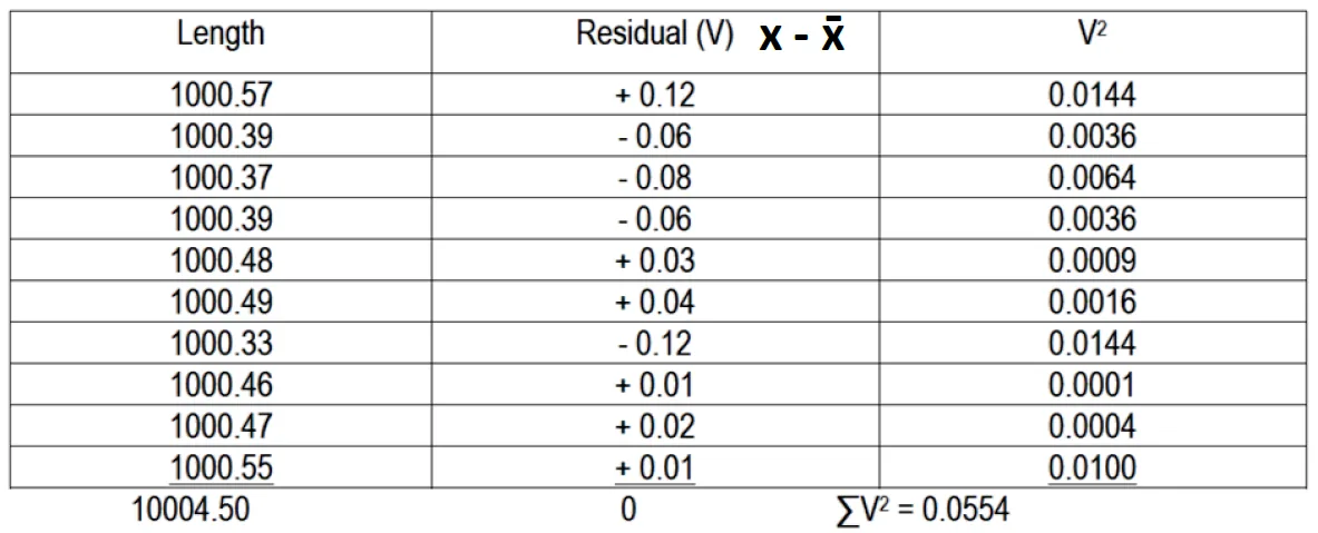
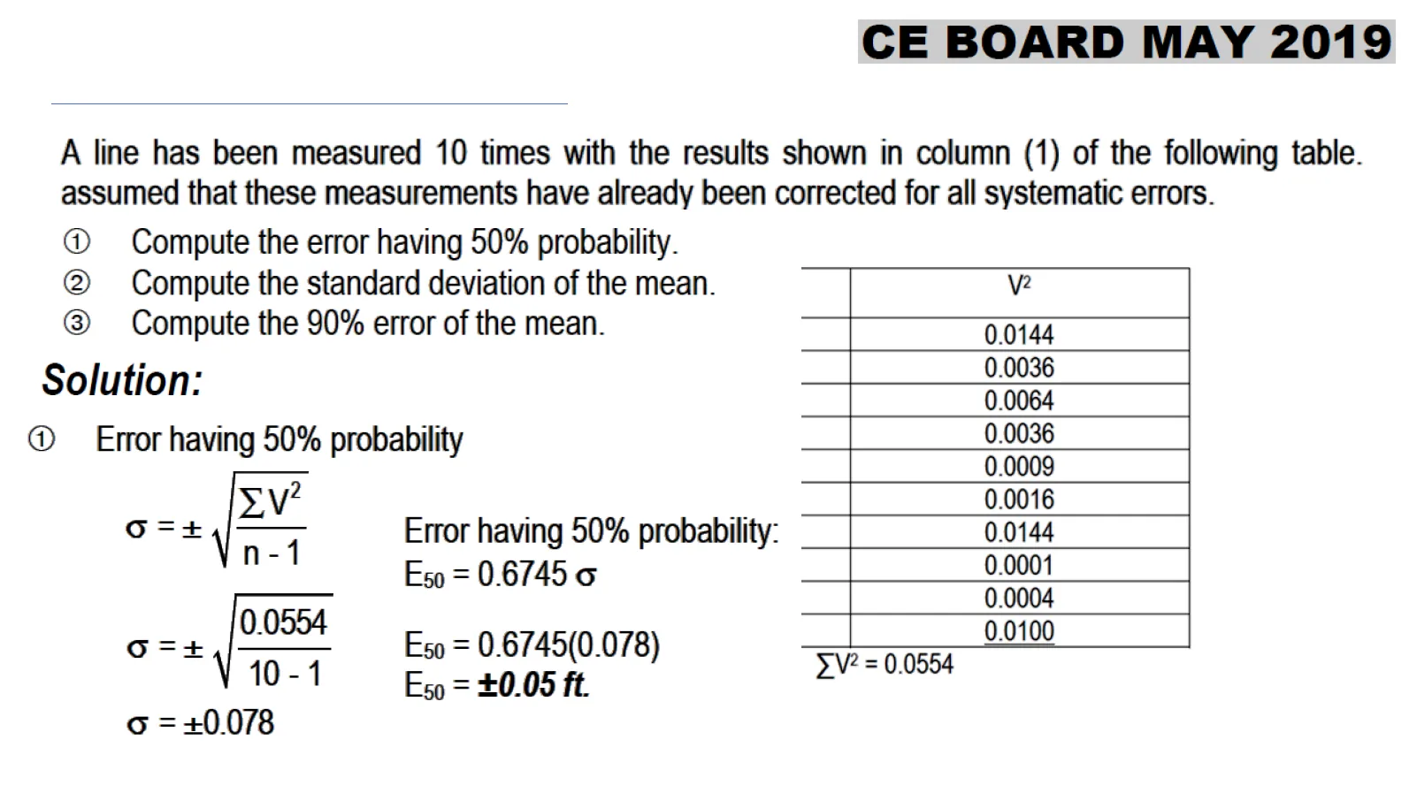
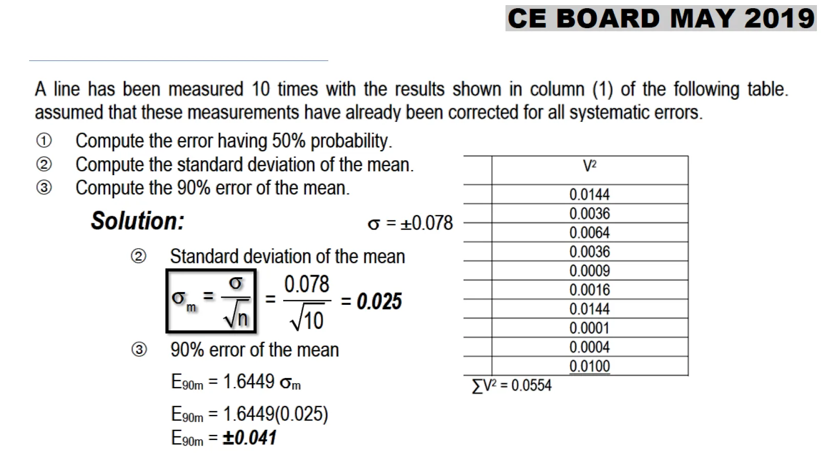
Problem 5:

CE Board Exam May 2019
A line has been measured 10 times with the results shown in column 1, assuming that the measurements have already been corrected for all systematic errors.
1. Compute the error having 50% probability
2. Compute the standard deviation of the mean.
3. Compute the 90% error of the mean.

See images: