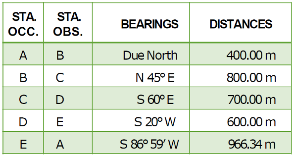
From the field notes of a closed traverse shown:
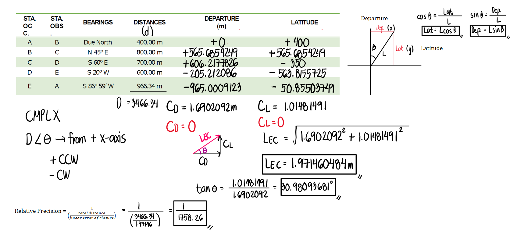
a. Compute the error of closure
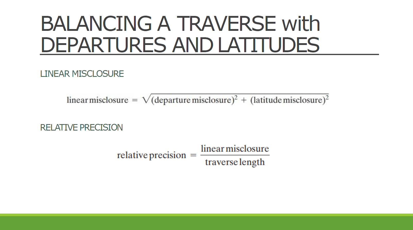
b. Compute the relative precision of the traverse
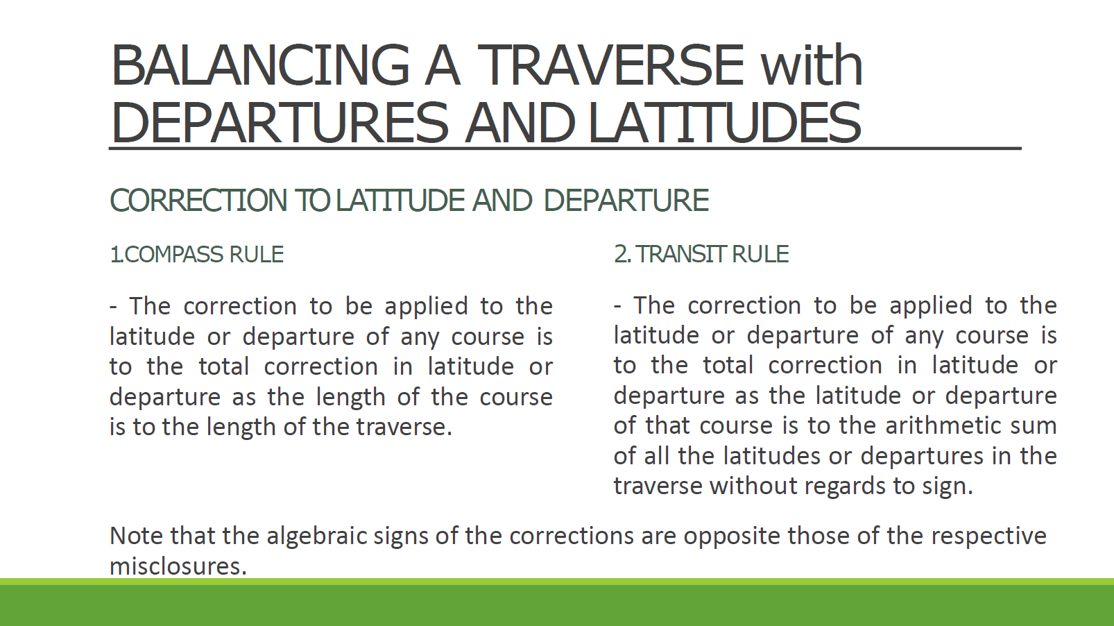
c. Compute the adjusted distances and bearings of the lines using the compass rule


To model our figure, let us first sketch each line separately.
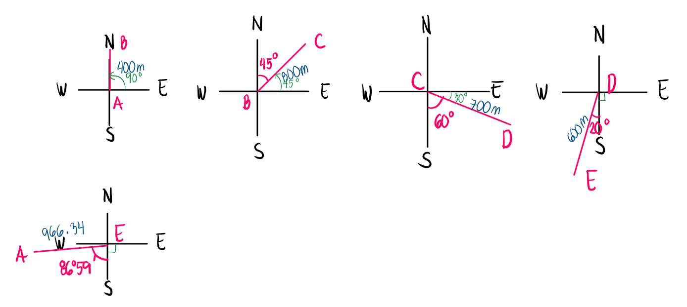
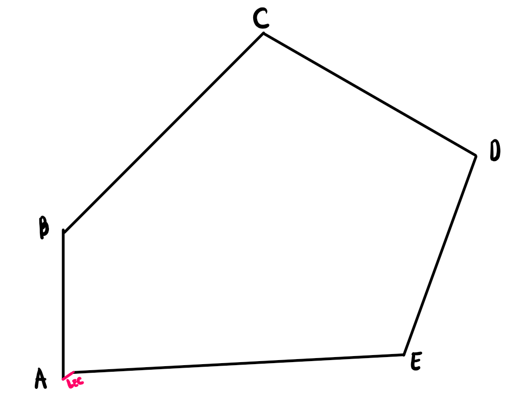
Connecting all of the lines, we obtain the following figure. If one models the figure using AutoCad, line EA will not yet connect back to point A. There will be some gap, and this gap between point A and E is called the linear error of closure.
The concept utilized here is similar to that of resultants in Statics of Rigid Bodies. The line that connects the first point (A) and the last point (E) is the resultant if we talk about forces. In the context of surveying, however, this is referred to as the linear error of closure.
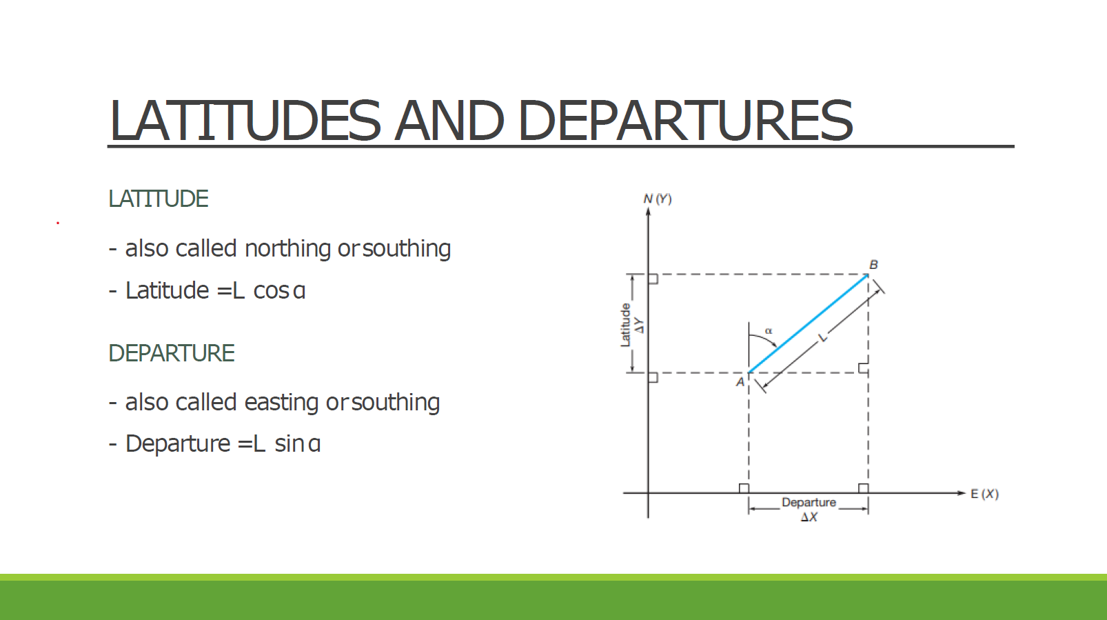
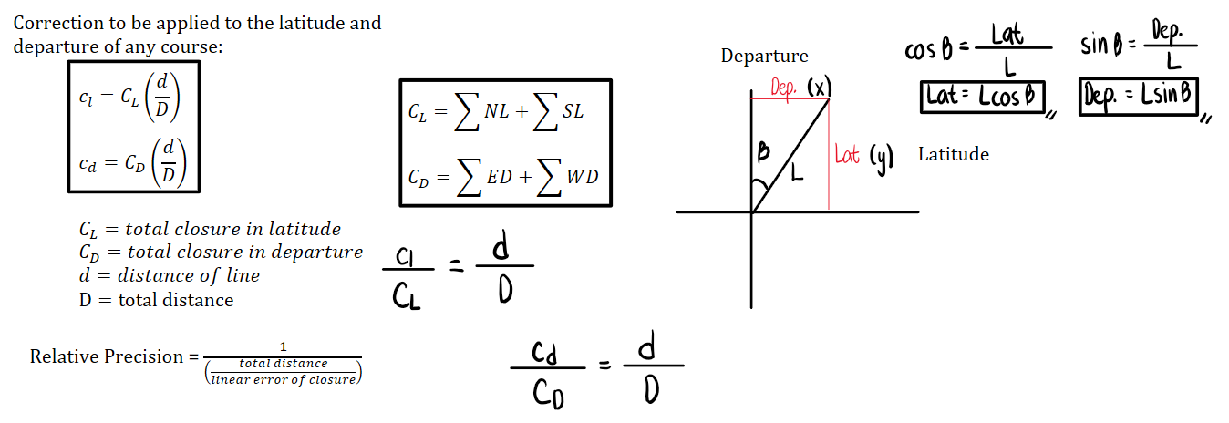
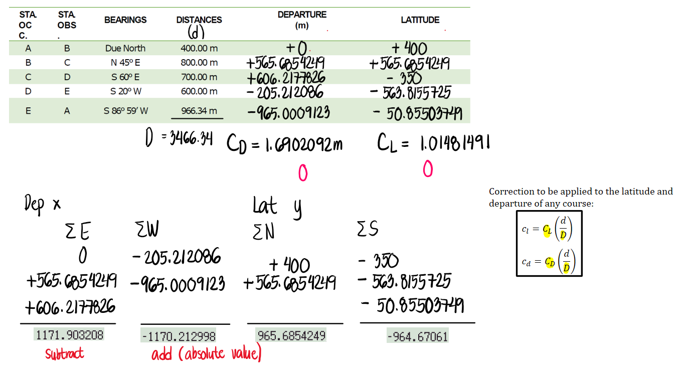
The linear error of closure will simply be the hypotenuse of the triangle formed by the sum of the departures and latitudes. We also solve the angle using the relationship between the two sides. Note that CD and CL are both positive. Hence, we subtract the corrections to the departures and latitudes so that the new summation will result to zero.
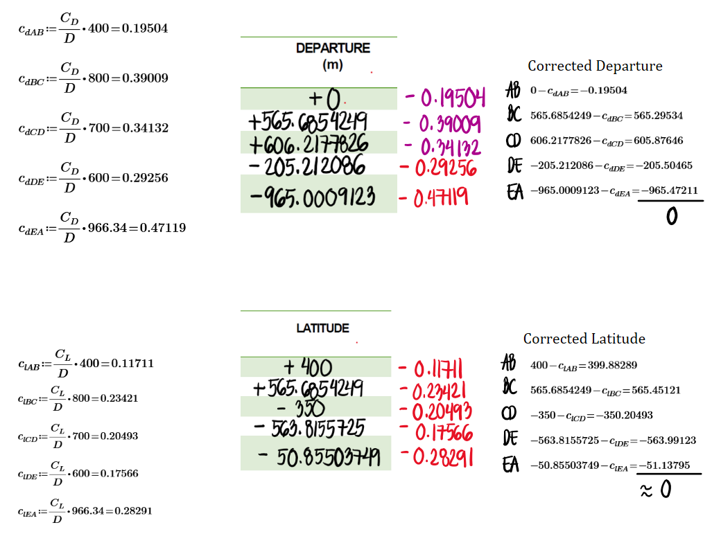
Let us focus on the sum of east departures. The result is 1171.903208m. Then, for the sum of west departures, the result is -1170.212998m. Notice that if we add both of them, the result will not be zero. To "close" the traverse, the sum should be equal to zero. To do this, we take away some value from 1171.903208m and add to the magnitude of -1170.212998m. Only when both east and west departures become equal in magnitude and opposite in signs will the correction become zero. To simplify the process, if CD or CL is positive, we subtract the corrections to each departure or latitude. If CD or CL is negative, we add the corrections to each departure or latitude.
The corrected departures and latitudes are shown below. Note that to check whether all calculations are correct, we can sum up the new departures and latitudes. If the result is zero, then the new linear of closure will also be zero.
Below are the corrected distances and bearings. If one models the following data using AutoCad, line EA will connect back to point A with a linear error of closure virtually equal to zero.

Compute the adjusted distances and bearings of the lines using the transit rule


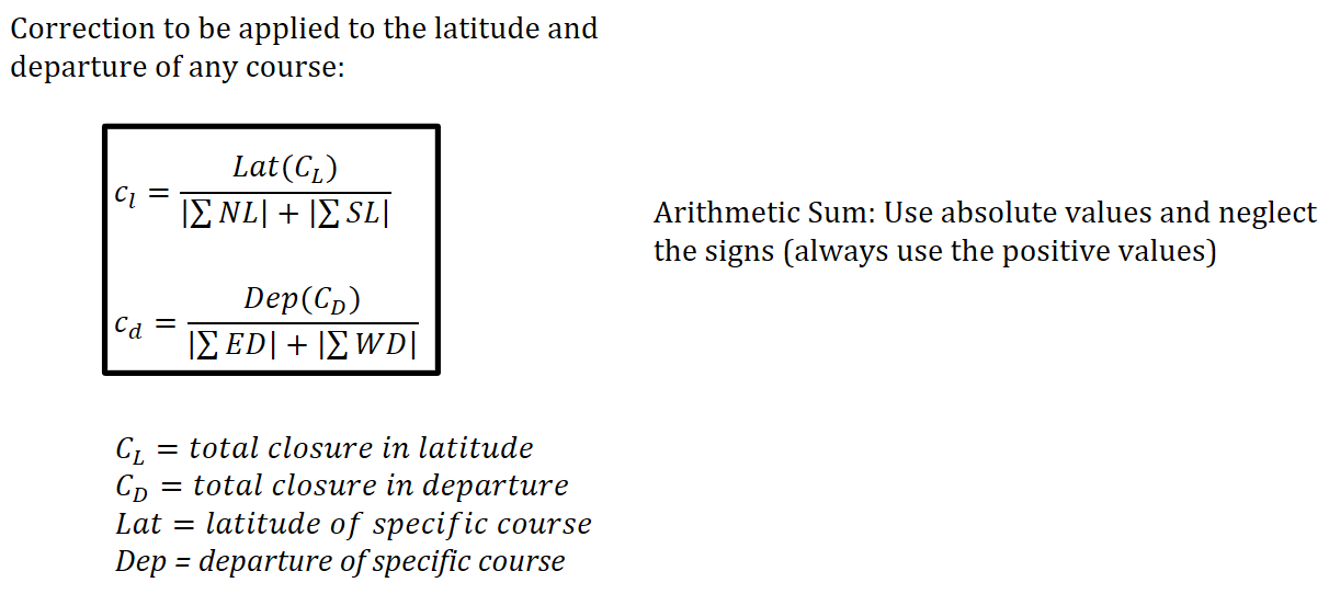
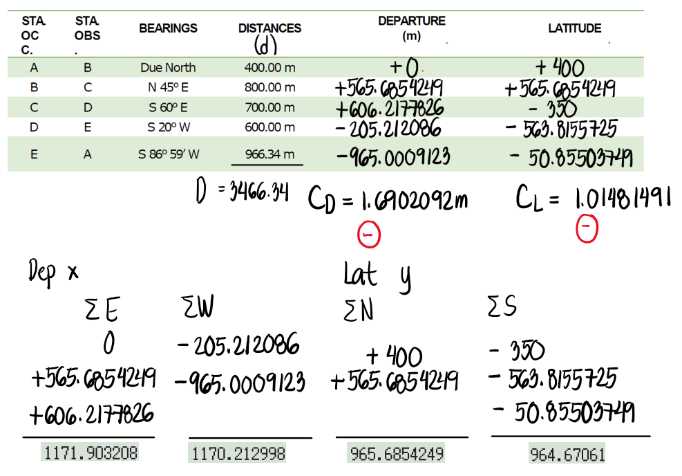
Here we use the arithmetic sum (neglecting the signs and using only the absolute values) when we sum up the north and south latitudes as well as the east and west departures.
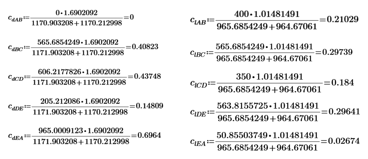
Next, we use the correction formula for transit rule for each departure and latitude.
When we sum up the corrected departures and latitudes, the result must be zero. This signifies that the linear error of closure will also be zero, which ensures that the traverse is closed.
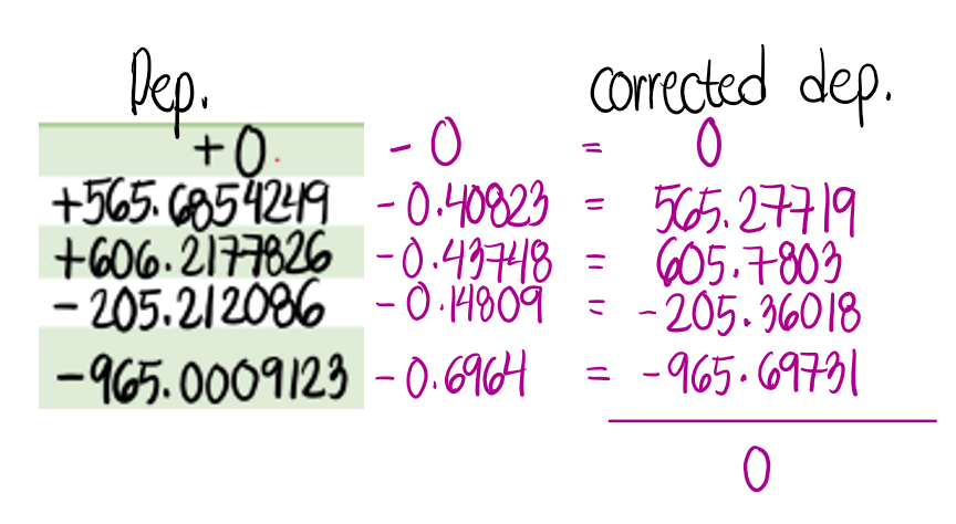
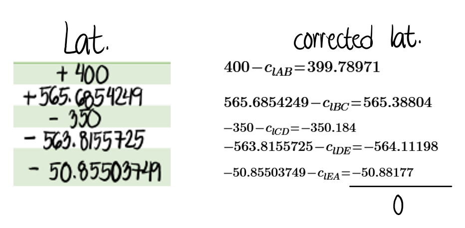
The corrected lengths and bearings using the transit rule are shown below. Note that the results here differ from the compass rule, but only by a small amount.

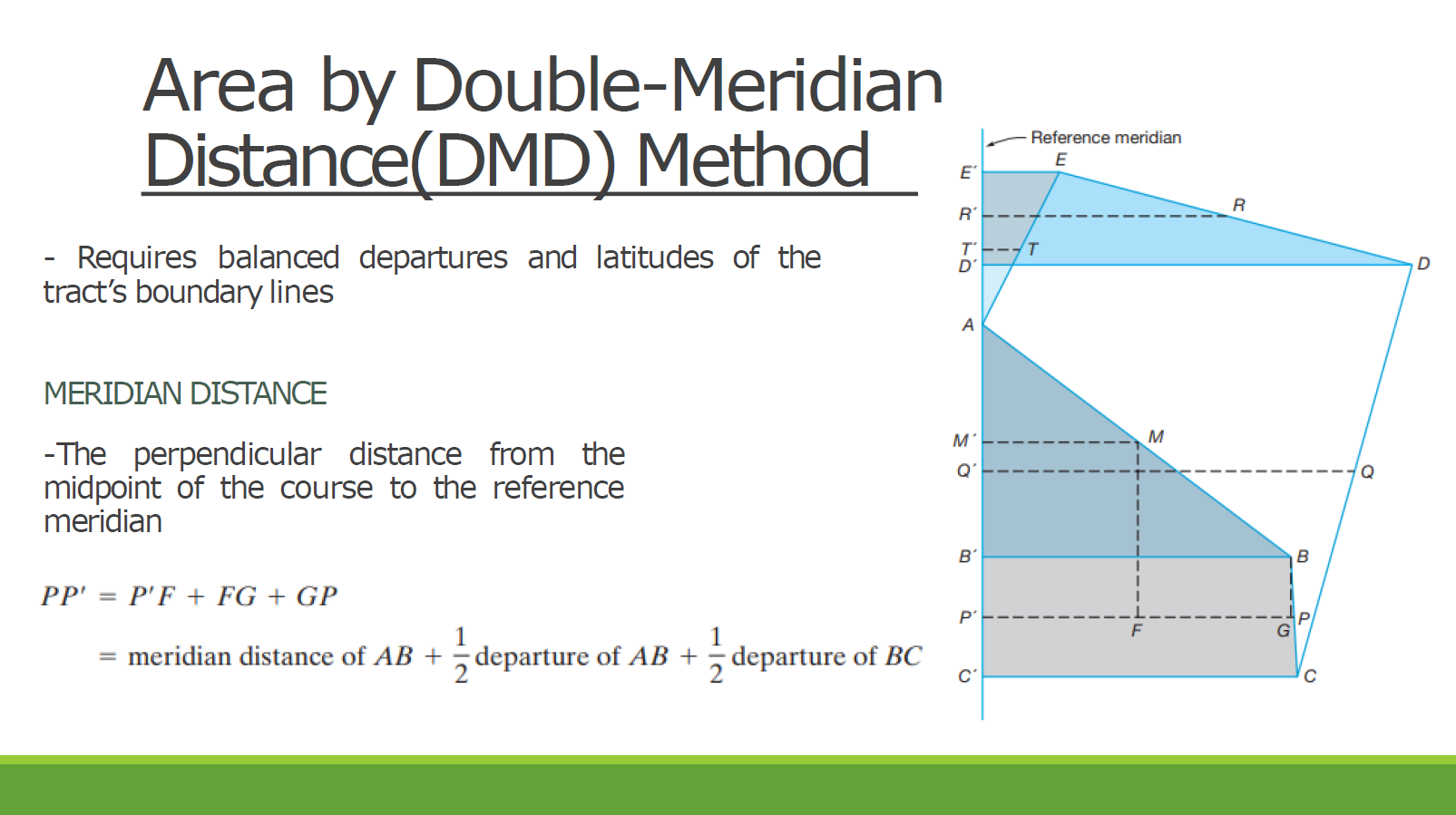
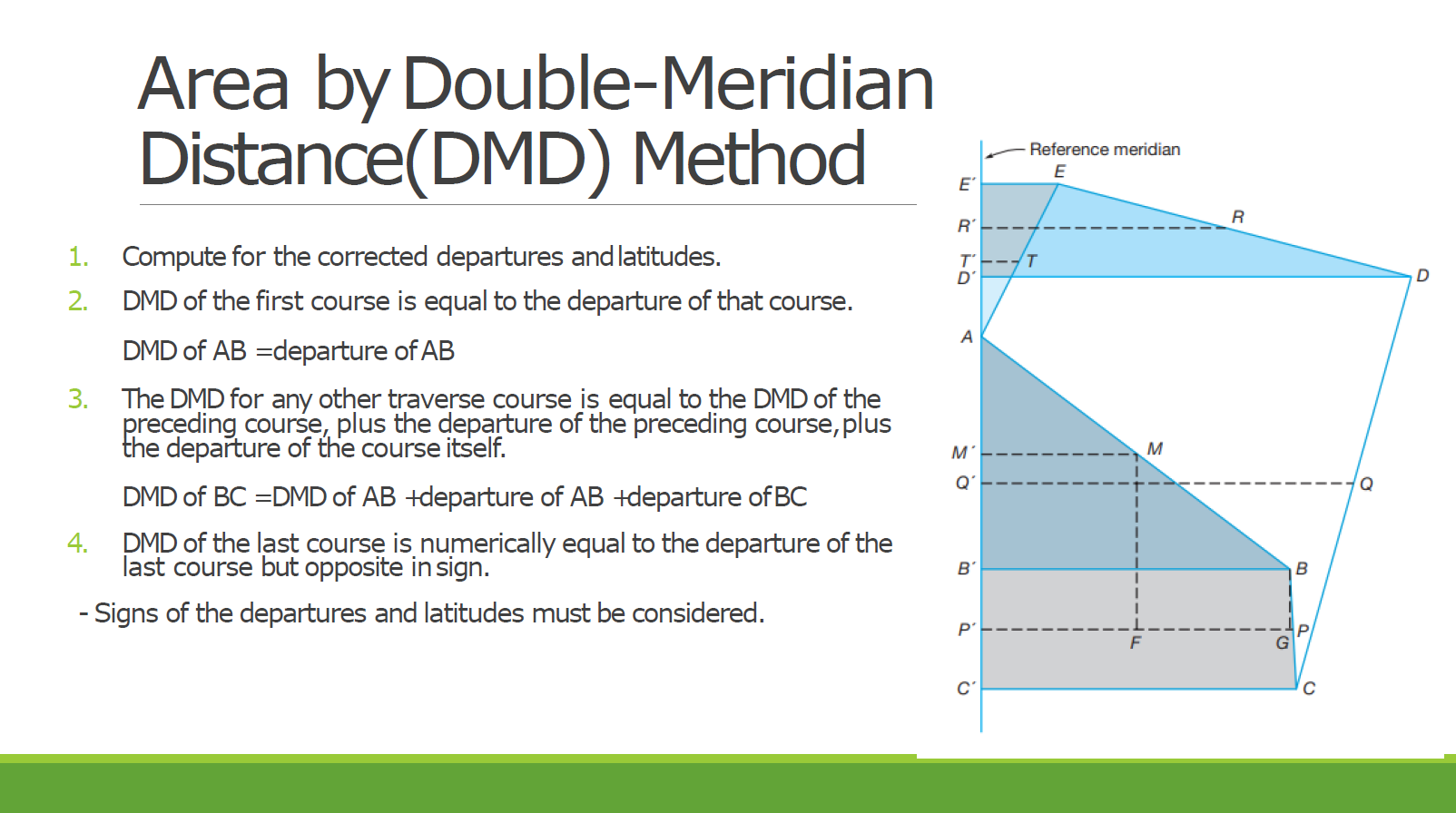
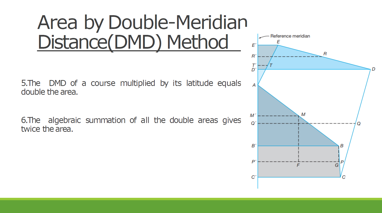
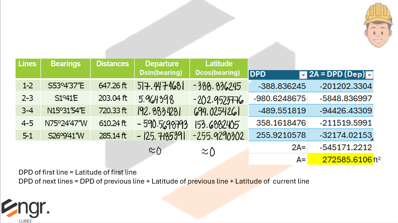
Given below is the technical description of lot 2081, Cebu Cadastre. Compute the area of the lot (in hectares) by DMD method.
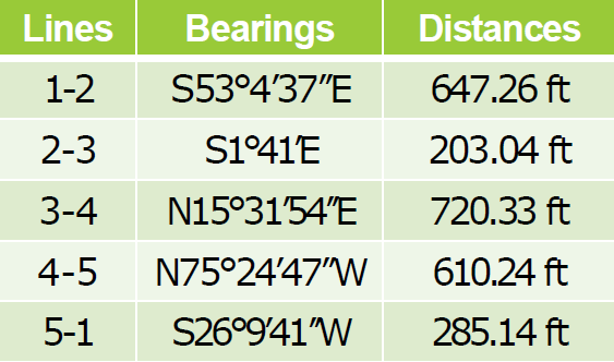


Note here that the DMD of the last line must be numerically equal to the departure of that line, but with opposite sign. However, there is some discrepancy due to the linear error of closure not being exactly zero.
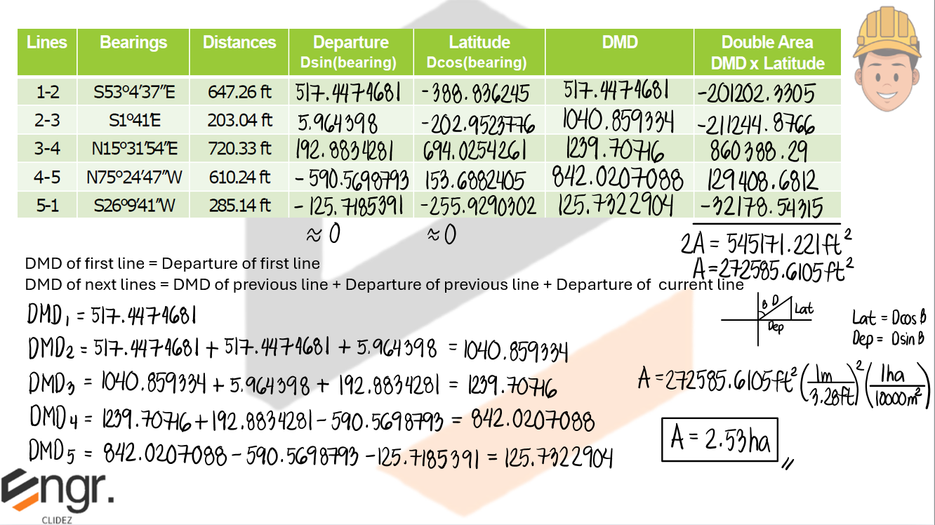


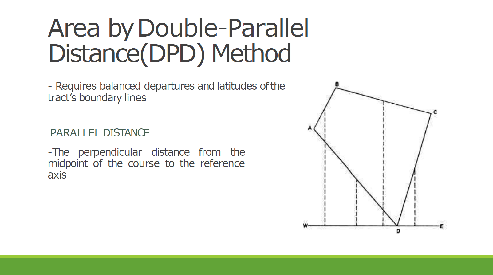
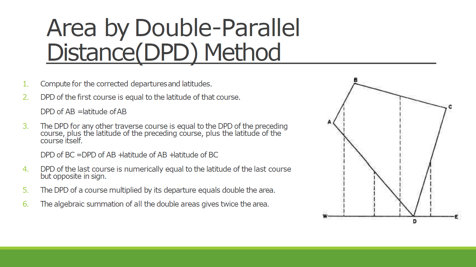
Resolve the area in Problem 3 using DPD method.


Note here that the DPD of the last line must be numerically equal to the latitude of that line, but with opposite sign. However, there is some discrepancy due to the linear error of closure not being exactly zero.


Refer to the image shown:


See images:


Refer to the image shown:


See images:


Refer to the image shown:


See images:


Refer to the image shown:


See images:


