CE Board Exam Randomizer

Vertical Curves: Symmetrical Parabolic Curve

In highway practice, an abrupt change in the vertical direction of moving vehicles should be avoided. To provide a gradual change in vertical direction, a parabolic vertical curve is adopted because its slope varies at a constant rate with respect to horizontal distance.

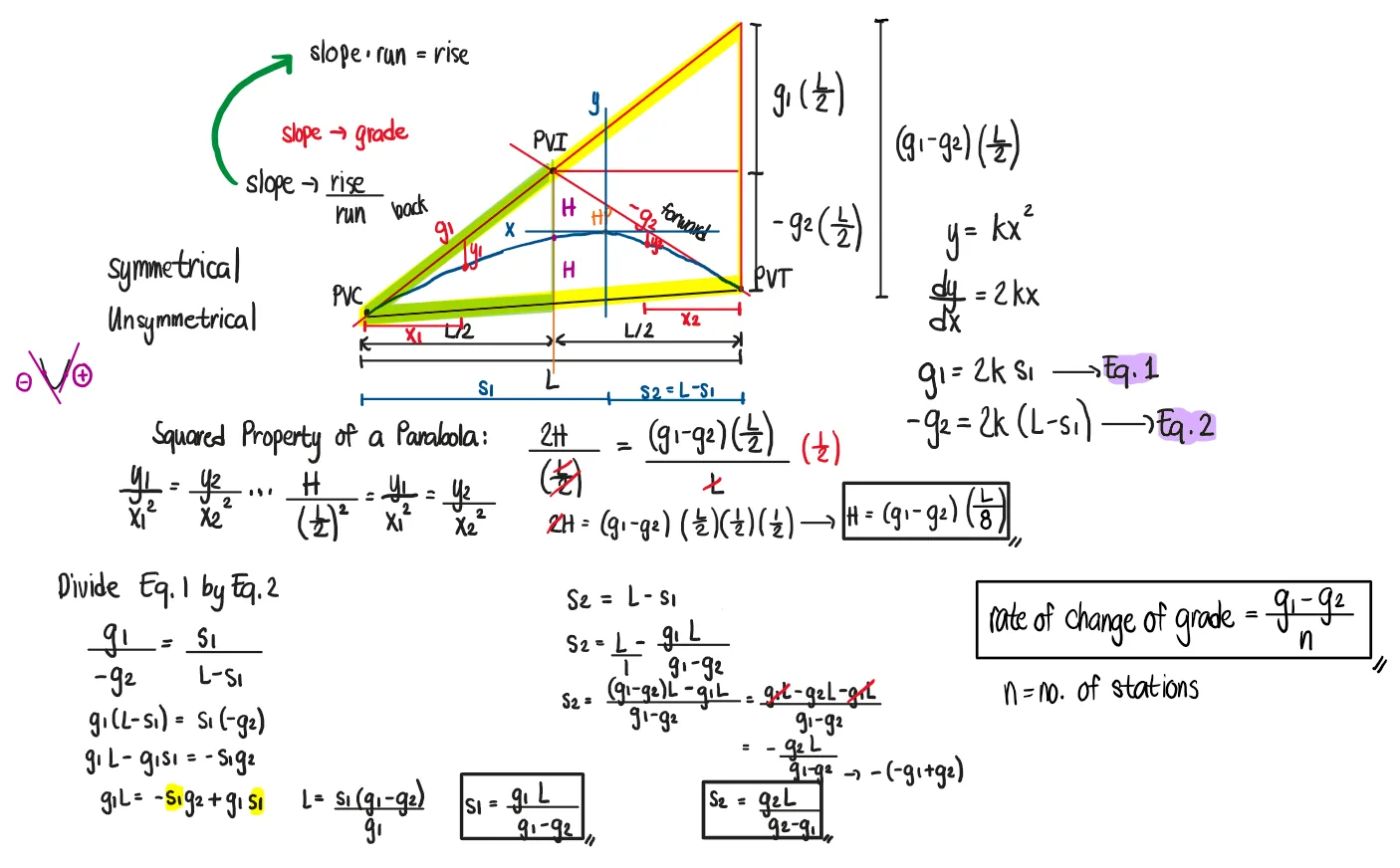
1. The vertical offsets from the tangent to the curve are proportional to the squares of the distances from the point of tangency.
2. The curve bisects the distance between the vertex and the midpoint of the long chord.
3. If the algebraic difference in the rates of grade of the two slopes is positive, i.e., $(g_1-g_2)>0$, we have a summit curve. Otherwise, we have a sag curve.
4. The length $L$ of a vertical parabolic curve refers to the horizontal distance from the PC to the PT.
5. The stationing of vertical parabolic curves is measured not along the curve, but along a horizontal line.
6. For a symmetrical parabolic curve, the number of stations to the left must be equal to the number of stations to the right of the intersection of the slopes (forward and backward tangents).
7. The slope of the parabola varies uniformly along the curve.
8. The maximum offset $H$ is $\tfrac{1}{8}$ of the product of the algebraic difference between the two rates of grade and the length of curve.

   Summary of Formulas in Symmetrical Parabolic Curves

   Location of the highest point from PC:

   $$s_1=\frac{g_1L}{g_1-g_2}$$

   Location of the highest point from PT:

   $$s_2=\frac{g_2L}{g_2-g_1}$$
   $$H=(g_1-g_2)\cdot\frac{L}{8}$$
   $$\text{rate of change of grade}=\frac{g_1-g_2}{n}$$
   n = no. of stations
   1 station = 100ft in English Units
   1 station = 20m in S.I. Units

   Grade Diagram for Vertical Parabolic Curves

   A grade diagram is a graphical representation of how the slope (grade) varies along the horizontal distance of the curve. Since the slope of a parabolic curve varies uniformly, the grade diagram is a straight line.

   Steps in Constructing the Grade Diagram

   1. Determine the algebraic difference in grade:
      Compute
      $$ A = g_2 - g_1 $$
      where $g_1$ is the initial grade and $g_2$ is the final grade.
   2. Determine the length of curve:
      Let $L$ be the horizontal length from PC to PT.
   3. Compute the rate of change of grade:
      $$ r = \frac{g_2 - g_1}{L} $$
      This represents the constant rate at which the slope changes per unit horizontal distance.
   4. Establish horizontal axis:
      Lay out the horizontal distance from PC (0) to PT ($L$).
   5. Plot the initial and final grades:
      At $x = 0$, ordinate = $g_1$. At $x = L$, ordinate = $g_2$.
   6. Join the two grade points with a straight line:
      Since the slope varies uniformly, the grade diagram is linear.

   ---

   Important Interpretations of the Grade Diagram

   • The ordinate of the grade diagram at any horizontal distance $x$ represents the slope (grade) of the curve at that point.
   • The area under the grade diagram between two points represents the difference in elevation between those two points.

   Mathematically, since grade is defined as the rate of change of elevation:

   $$ g = \frac{dy}{dx} $$

   The elevation difference between two points is therefore:

   $$ \Delta y = \int g \, dx $$

   Thus, the grade diagram is essentially a graphical integration tool — the area under the grade line gives the vertical change in elevation.

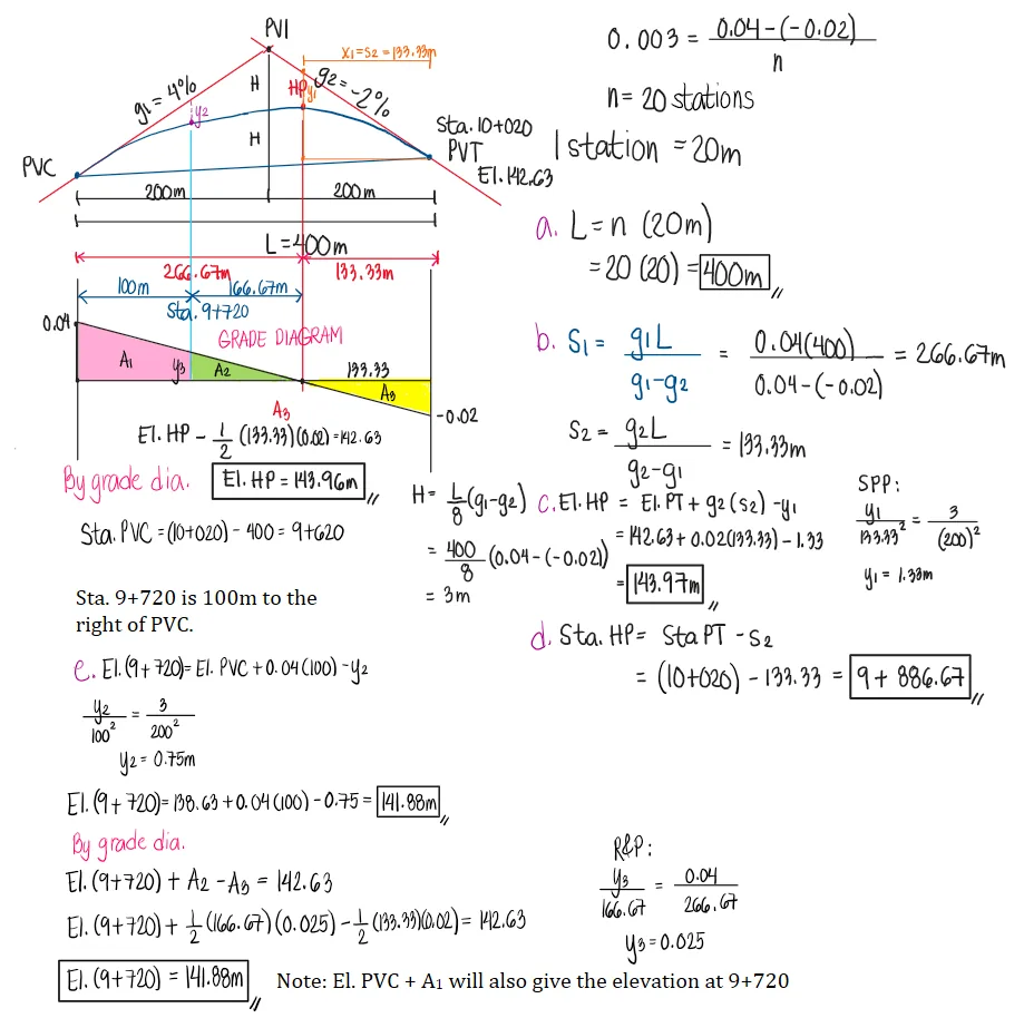
Problem: Symmetrical Vertical Summit Curve with Allowable Rate of Change of Grade

A symmetrical vertical summit curve has tangents of +4% and -2%. The allowable rate of change of grade is 0.3% per meter station. The stationing and elevation of PT is 10+020 and 142.63m, respectively.
a. Compute the length of curve.
b. Compute the distance of the highest point of the curve from the PC.
c. Compute the elevation of the highest point of the curve.
d. Determine the stationing of the highest point of the curve.
e. Determine the elevation of a point at station 9+720.

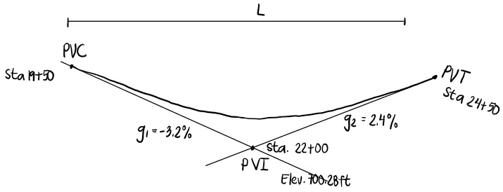
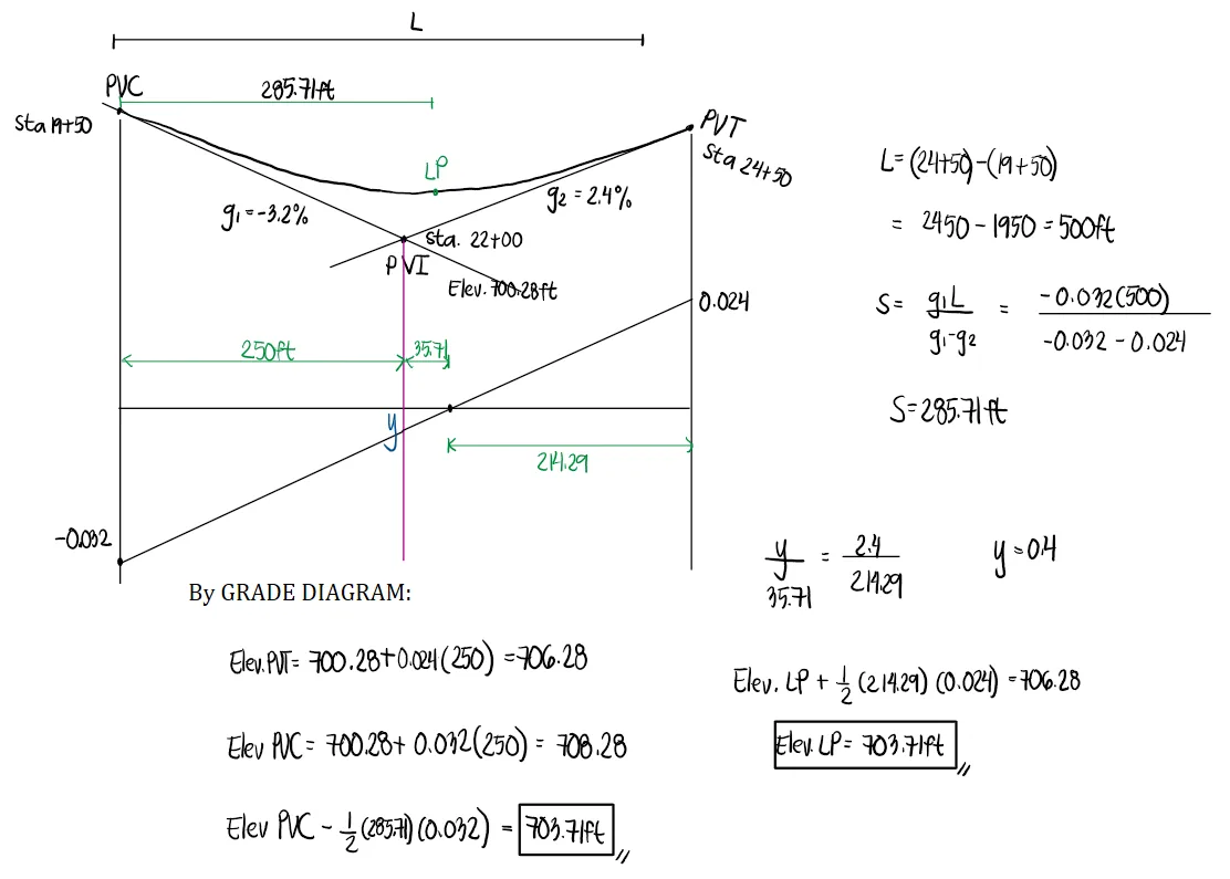
Problem: Sag Vertical Curve with English Units

A symmetrical sag vertical curve is shown. Determine the elevation of the lowest point of the curve.

Problem: Symmetrical Sag Vertical Curve | Invert Elevation and all Possible Cases of the Grade Diagram

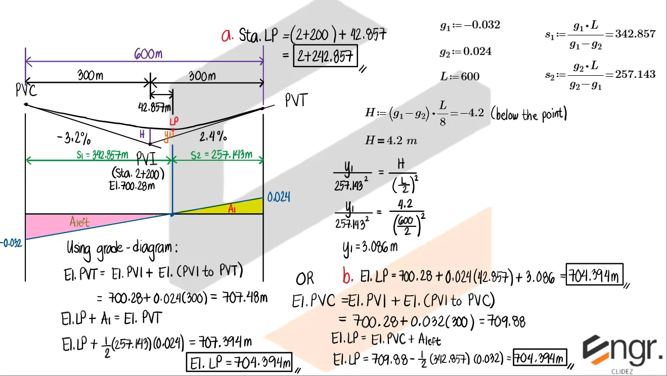
A symmetrical sag vertical curve has a back tangent grade of -3.2% and a forward tangent grade of 2.4%, intersecting at the point PVI whose stationing is 2+200 at an elevation of 700.28m. The stationing of PVC is 1+900.
a. At what station should the cross-drainage pipes be situated?
b. What is the elevation of the lowest point?
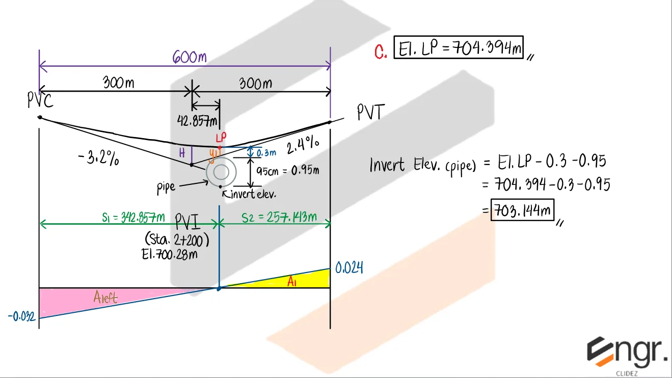
c. If the overall outside dimensions of the reinforced concrete pipe to be installed is 95cm, and the top of the culvert is 0.3m below the subgrade, what will be the invert elevation (elevation of the lowest point of the pipe)?
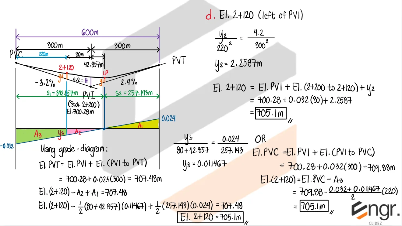
d. Determine the elevation at station 2+120.
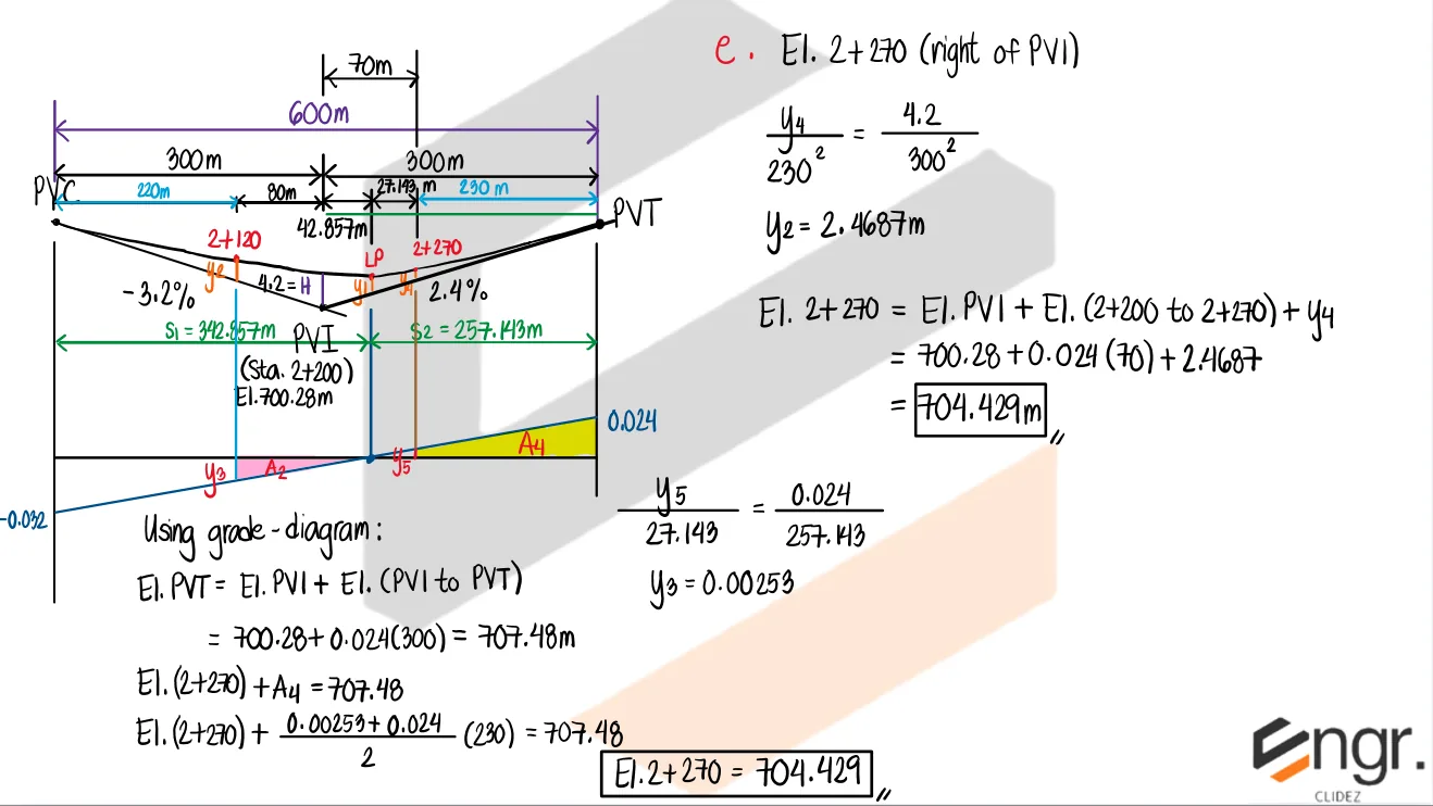
e. Determine the elevation at station 2+270.